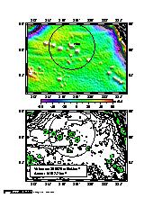
#!/bin/bash
#		GMT EXAMPLE 18
#
#		@(#)job18.bash	1.9  03/11/99
#
# Purpose:	Illustrates volumes of grids inside contours and spatial
#		selection of data
# GMT progs:	gmtset, gmtselect, grdclip, grdcontour, grdgradient, grdimage,
# Unix progs:	$AWK, cat, rm
#
# Get Sandwell/Smith gravity for the region
#img2latlongrd world_grav.img.7.2 -R-149/-135/52.5/58 -Gss_grav.grd -T1

# Use spherical projection since SS data define on sphere
gmtset ELLIPSOID Sphere

# Define location of Pratt seamount
echo "-142.65	56.25" > pratt.d

# First generate gravity image w/ shading, label Pratt, and draw a circle
# of radius = 200 km centered on Pratt.

makecpt -Crainbow -T-60/60/10 -Z > grav.cpt
grdgradient ss_grav.grd -Nt1 -A45 -Gss_grav_i.grd
grdimage ss_grav.grd -Iss_grav_i.grd -JM5.5i -Cgrav.cpt -B2f1 -P -K -X1.5i -Y5.85i > example_18.ps
pscoast -R-149/-135/52.5/58 -JM -O -K -Di -G160 -W0.25p >> example_18.ps
psscale -D2.75i/-0.4i/4i/0.15ih -Cgrav.cpt -B20f10/:mGal: -O -K >> example_18.ps
$AWK '{print $1, $2, 12, 0, 1, "LB", "Pratt"}' pratt.d | pstext -R -JM -O -K -D0.1i/0.1i >> example_18.ps
$AWK '{print $1, $2, 0, 200, 200}' pratt.d | psxy -R -JM -O -K -SE -W0.25p >> example_18.ps

# Then draw 10 mGal contours and overlay 50 mGal contour in green

grdcontour ss_grav.grd -JM -C20 -B2f1WSEn -O -K -Y-4.85i -U/-1.25i/-0.75i/"Example 18 in Cookbook" >> example_18.ps
grdcontour ss_grav.grd -JM -C10 -L49/51 -O -K -Dsm -Wc0.75p/0/255/0 >> example_18.ps
pscoast -R -JM -O -K -Di -G160 -W0.25p >> example_18.ps
$AWK '{print $1, $2, 0, 200, 200}' pratt.d | psxy -R -JM -O -K -SE -W0.25p >> example_18.ps
\rm -f sm_*[0-9].xyz	# Only consider closed contours

# Now determine centers of each enclosed seamount > 50 mGal but only plot
# the ones within 200 km of Pratt seamount.

# First make a simple $AWK script that returns the average position
# of a file with coordinates x, y (remember to escape the $ sign)

cat << EOF > center.awk
BEGIN {
	x = 0
	y = 0
	n = 0
}
{
	x += \$1
	y += \$2
	n++
}
END {
	print x/n, y/n
}
EOF

# Now determine mean location of each closed contour and
# add it to the file centers.d

\rm -f centers.d
for file in sm_*.xyz
do
	$AWK -f center.awk $file >> centers.d
done

# Only plot the ones within 200 km

gmtselect -R -JM -C200/pratt.d centers.d > $$
psxy $$ -R -JM -O -K -SC0.04i -G255/0/0 -W0.25p >> example_18.ps
psxy -R -JM -O -K -ST0.1i -G255/255/0 -W0.25p pratt.d >> example_18.ps

# Then report the volume and area of these seamounts only
# by masking out data outside the 200 km-radius circle
# and then evaluate area/volume for the 50 mGal contour

grdmath -R -I2m -F -142.65 56.25 GDIST = mask.grd
grdclip mask.grd -Sa200/NaN -Sb200/1 -Gmask.grd
grdmath ss_grav.grd mask.grd MUL = tmp.grd
area=`grdvolume tmp.grd -C50 -Sk | cut -f2`
volume=`grdvolume tmp.grd -C50 -Sk | cut -f3`

psxy -R -JM -A -O -K -L -W0.75p -G255 << EOF >> example_18.ps
-148.5 52.75
-140.5	52.75
-140.5	53.75
-148.5	53.75
EOF
pstext -R -JM -O << EOF >> example_18.ps
-148 53.08 14 0 1 LM Areas: $area km@+2@+
-148 53.42 14 0 1 LM Volumes: $volume mGal\264km@+2@+
EOF

# Clean up

\rm -f $$ grav.cpt sm_*.xyz *_i.grd tmp.grd mask.grd pratt.d center* .gmt*